PEER research on seismic performance assessment is approaching the end of its second year. Much has been accomplished, but the end of the road still looks far away. In this brief article we describe the foundation on which performance assessment can be based, and the major challenges to the PEER research community on the way to expected success.

Proposed Probabilistic Foundation

The following scheme is presented as an effective foundation for the development of performance-based guidelines. It suggests a generic structure for coordinating, combining, and assessing the many considerations implicit in performance-based seismic assessment and design.

The suggested foundation in its generalized form assumes that the basis for assessing the adequacy of the structure or its design will be a vector of certain key Decision Variables, , such as the annual earthquake loss and/or the exceedance of one or more limit states (e.g., collapse). These can only be predicted probabilistically. Therefore the specific objectives of engineering assessment analyses are in effect quantities such as , the mean annual frequency1 (MAF) of the loss exceeding x dollars, or such as , the MAF of collapse, or more formally the mean annual frequency that the collapse indicator variable2, , exceeds 0.

Then, the practical and natural analysis strategy involves the expansion and/or "disaggregation" of the MAF, , in terms of structural Damage Measures, , and ground motion Intensity Measures, , which can be written symbolically as

(1)

Here is the probability that the (vector of) decision variable(s) exceed specified values given (i.e., conditional on knowing) that the engineering Damage Measures (e.g., the maximum interstory drift, and/or the vector of cumulative hysteretic energies in all elements) are equal to particular values. Further, is the probability that the Damage Measure(s) exceed these values given that the Intensity Measure(s) (such as spectral acceleration at the fundamental mode frequency, and/or spectral shape parameters and/or duration) equal particular values. Finally is the MAF of the Intensity Measure(s).

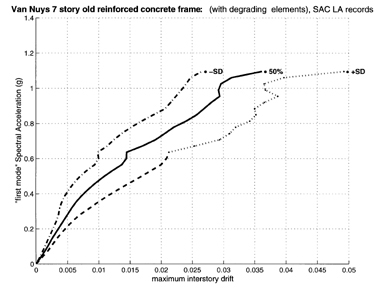
We note that is in fact just a seismic hazard curve, the determination of which is accomplished by conventional Probabilistic Seismic Hazard Analysis (PSHA) (or in the vector case, a more advanced PSHA). Secondly, the estimation of is the objective of linear and nonlinear dynamic analysis or seismic "demand analysis" under (the multiple possible) accelerograms with a given intensity level. For example, Figure 1 shows in the form of the median as well as 16th- and 84th-percentiles of maximum interstory drift (DM) given the spectral acceleration at the first-mode period (IM) for a model of the Van Nuys Holiday Inn RC moment-resisting frame. (These curves are the result of incremental dynamic analyses of 30 records.) The choice of Damage Measures should be driven by how effectively they "predict" the Decision Variables, which is captured by the breath of the probability distribution . Examples of when the DV is a binary damage state indicator variable are various "fragility curves." In the case of nuclear power plant seismic Probabilistic Risk Assessments (PRAs), the fragility is the probability associated with exceeding the random capacity of a structure or plant damage state (e.g., core melt), and in the case of the more recent HAZUS software, it is the likelihood of a given discrete loss state3. The authors believe that continuous decision (loss) variables may prove effective in the latter case4.

Figure 1: Van Nuys 7 Story old reinforced concrete frame: (with degrading elements), SAC LA records

Inspection of the generic equation above5 reveals that it "de-constructs" the assessment problem into the three basic elements of (1) hazard analysis, (2) dynamic demand prediction, and (3) failure or loss estimation, by introducing the two "intermediate variables," and . Then it re-couples the elements by integration over all levels of the selected intermediate variables.6 This integration implies that in principle7 the conditional probabilities and must be assessed parametrically over a suitable range of and levels.

The choice of appropriate intermediate variables is part of the science and art of successful engineering analysis. Of course, simplicity favors scalar measures, but the selection should be done thoughtfully. For example, choosing PGA for the intensity measure may be initially appealing, but implies that the distribution G(DM|IM) may have a very broad variability for all but very short period structures. This in turn means that a large sample of records and nonlinear analyses will be required to estimate G(DM|IM) with sufficient confidence. Further, without very careful record selection or weighting of the results one may easily obtain inaccurate results that for instance, fail to reflect the correct likelihood of the longer period spectral content that is important for taller buildings. A well-selected spectral ordinate (e.g., at the fundamental period) or an appropriate vector (e.g., PGA and, say, at a period of 2 sec.) can improve this situation.

Further, to avoid complexity one would like intermediate variables to be selected such that conditioning information need not be "carried forward." (Indeed, Equation 1 is intentionally written under the implicit assumption that, given , is conditionally independent of . Otherwise should appear after the in the first factor.) So, for example, the measures of damage should be selected so that the decision variables do not also vary with intensity, once the damage measure is specified, Similarly, one should chose the intensity measures () so that the dynamic response, (), once it is given, is not also further influenced by, say, magnitude or distance8, which have already been integrated into the determination of (through incidentally an expansion and integration parallel to Equation 1).

Space limitations preclude providing more detailed examples in this article. The reader is instead referred to the SAC seismic guidelines for SMRF buildings and to the draft ISO seismic guidelines for fixed offshore jacket structures for examples that follow the scheme outlined here. The scheme is sufficiently general to be applicable to performance assessment with discrete decision variables (targeted performance levels or discrete loss states) as well as with continuous decision (loss) variables.

Challenge for PEER Researchers

We believe that the aforementioned scheme is sufficiently general to form the basis for PEER's various efforts on seismic performance assessment. The challenge is not to invent a new basis but to provide a direction toward which the various PEER research efforts should converge. At this time PEER researchers are pursuing and evaluating various options that present themselves as valuable alternatives.

One option is to develop a general methodology for estimating the annualized expected costs associated with the seismic risk (initial, maintenance, insurance, etc., plus annualized earthquake losses), with consideration of constraints imposed by society (e.g., tolerable annual probability of exceeding a life-threatening performance state [e.g., partial or complete collapse]) and, possibly, specific constraints imposed by the owner (e.g., acceptable annual probability of having to shut down for more than x days). This building/bridge specific loss estimation option, which should be "compatible" with seismic retrofit projects and new designs, is very attractive because it permits an evaluation of design (or retrofit) alternatives and provides the information the owner is most interested in. The question is whether this option can be brought to a sufficiently objective level to acquire the confidence of engineers and owners.

The second basic option is the development of a methodology that focuses on specific performance levels (which may range from continuous operation to collapse prevention) and an acceptable annual probability of exceeding these levels (the "performance objective" approach advocated in present guidelines [FEMA 273 and SEAOC Vision 2000]). In essence, this approach considers performance levels the same way as constraints are considered in the first option. This approach can be based on an LRFD-like format (capacities > demands). The open question is how to quantify acceptable performance (or capacities) at the various levels. Much work has been done in quantifying drift capacities for collapse, but other performance levels have not yet been addressed in a quantitative manner.

The second set of options may be considered as a subset of the first one. It remains to be seen if, by itself, the second set satisfies the needs of owners and society. Soon PEER may have to decide which option to pursue in detail.

The choice of an option will also depend on the ability to develop procedures, data, and tools necessary for implementation. This may be the biggest challenge for PEER researchers. The foundation outlined previously relies equally on cost estimation, hazard analysis, and structural analysis. In all three aspects much data and knowledge acquisition are needed.

The final challenge for PEER researchers is not in predicting performance or in estimating losses, but in contributing effectively to the reduction of losses and the improvement of safety. We must never forget this. It is easy to get infatuated with numbers and analytical procedures, but neither is useful unless it contributes to this final challenge.

C. Allin Cornell and Helmut Krawinkler
Professors of Civil and Environmental Engineering
Stanford University

1 The MAF is approximately equal to the annual probability for the small values of interest here. 2 An indicator variable, I, is a random variable that equals unity if the indicated event, e.g., collapse, occurs, and equals zero otherwise. It is simply a convenient, unifying way to represent random events as random variables. 3 More precisely these particular fragility curves are G(DV|IM), i.e., the intermediate variable DM has been ignored or ³integrated out.² 4 It should be noted that the expected annual loss can be found from . 5 The equation is nothing more than an example of the Total Probability Theorem. 6 It is this integration that requires that one obtain the likelihoods of specific levels by the differentiation implied by the two ³dıs² in Equation 1. 7 In practice this can often be avoided. 8 Note that this does not preclude selecting, say, magnitude, to be one of the elements of the IM vector, at the expense of increasing its length and hence the dimension of the analysis.